Elastic waves without potentials: from Chiappa's 2D benchmark to a 3D Fourier solution

While developing WaveCore, I keep returning to a simple question: how do I know that the waves it produces are the right ones?

An analytical benchmark is particularly useful here. It gives me a reference that is independent of a mesh, an element formulation or a time-stepping implementation. Chiappa et al. provide such a benchmark for elastic waves in a two-dimensional rectangular solid [1]. Their formulation introduces displacement potentials through the Helmholtz decomposition, solves the potential wave equations and reconstructs displacement.

I wanted to explore a different route: can I expand displacement itself in Fourier modes and solve directly for those coefficients? For this geometry and its sliding boundary conditions, the answer is yes. The calculation reduces to a small matrix for each spatial mode. Longitudinal and shear waves emerge from its eigenstructure, rather than being separated through potentials at the outset.

This is an alternative derivation of a classical solution, not a claim of a new physical model. Helmholtz decomposition remains useful in many settings. My point is narrower: it is an intermediate step we can avoid for this particular problem. A further attraction is how little the procedure changes when moving from two to three dimensions.

I will derive the 2D solution, establish its equivalence to Chiappa’s expressions, compare it with an independent finite-difference solver, and then extend the framework to a 3D Gaussian pulse. The 3D calculation is a benchmark for future WaveCore development; it is not a result from a 3D WaveCore implementation.

1. Define the problem before choosing the series

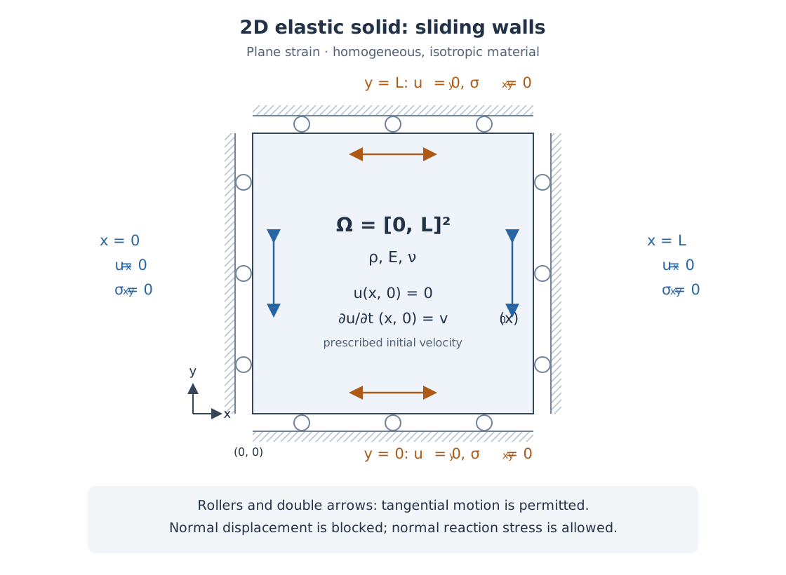Problem setup. Rollers permit tangential motion at each wall while blocking normal displacement. Normal reaction stress is allowed; the excitation comes from the prescribed initial velocity.

Consider a homogeneous, isotropic, linearly elastic solid. With no body force, its displacement satisfies

\[\rho\ddot{\mathbf u} =\mu\nabla^2\mathbf u+(\lambda+\mu)\nabla(\nabla\cdot\mathbf u).\]

Here $\rho$ is density, and the Lamé constants are

\[\mu=\frac{E}{2(1+\nu)},\qquad \lambda=\frac{E\nu}{(1+\nu)(1-2\nu)}.\]

The 2D problem is plane strain, so these are the three-dimensional material constants; this is not the plane-stress reduction.

Start with a square $\Omega=[0,L]^2$. Its walls permit tangential motion but prevent penetration. In addition to zero normal displacement, the tangential traction is zero:

Faces	Displacement constraint	Traction constraint
$x=0,L$	$u_x=0$	$\sigma_{xy}=0$
$y=0,L$	$u_y=0$	$\sigma_{xy}=0$

These are symmetry or sliding walls, not fully clamped walls and not traction-free boundaries. Normal reaction stress is allowed.

The initial conditions are

\[\mathbf u(\mathbf x,0)=\mathbf0,\qquad \dot{\mathbf u}(\mathbf x,0)=\mathbf v_0(\mathbf x).\]

The initial velocity supplies the excitation. We will first use Chiappa’s constant patch and later replace it with a Gaussian.

2. Expand displacement directly in 2D

Set $k_x=n\pi/L$ and $k_y=m\pi/L$. Choose

\[\begin{aligned} u_x(x,y,t)&=\sum_{n=1}^{\infty}\sum_{m=0}^{\infty} X_{nm}(t)\sin(k_xx)\cos(k_yy),\\ u_y(x,y,t)&=\sum_{n=0}^{\infty}\sum_{m=1}^{\infty} Y_{nm}(t)\cos(k_xx)\sin(k_yy). \end{aligned}\]

Each component has a sine in its own direction and a cosine in the other. The normal displacement is therefore zero at its walls. Also,

\[\sigma_{xy}=\mu(u_{x,y}+u_{y,x}) =-\mu\sum_{n,m}(k_yX_{nm}+k_xY_{nm})\sin(k_xx)\sin(k_yy),\]

which vanishes on all four faces. Every retained term satisfies the boundary conditions.

Substitute into the equations

First, a note on the notation: the $x$ in $u_x$ identifies the displacement component, whereas indices after a comma identify spatial derivatives. For example,

\[u_{x,xx}=\frac{\partial^2u_x}{\partial x^2},\qquad u_{x,yy}=\frac{\partial^2u_x}{\partial y^2},\qquad u_{y,xy}=\frac{\partial}{\partial y} \left(\frac{\partial u_y}{\partial x}\right).\]

A dot denotes a time derivative, so $\ddot u_x=\partial^2u_x/\partial t^2$. The Fourier modes are smooth, so the order of their mixed spatial derivatives can be exchanged.

Write out the vector equation component by component

In plane strain, $\mathbf u=(u_x,u_y,0)$ and the fields do not depend on $z$. The divergence is the scalar

\[\nabla\cdot\mathbf u=u_{x,x}+u_{y,y}.\]

Taking its gradient gives

\[\nabla(\nabla\cdot\mathbf u) =\begin{bmatrix} \partial_x(u_{x,x}+u_{y,y})\\ \partial_y(u_{x,x}+u_{y,y}) \end{bmatrix} =\begin{bmatrix} u_{x,xx}+u_{y,xy}\\ u_{x,xy}+u_{y,yy} \end{bmatrix}.\]

The vector Laplacian acts on each component separately:

\[\nabla^2\mathbf u =\begin{bmatrix} u_{x,xx}+u_{x,yy}\\ u_{y,xx}+u_{y,yy} \end{bmatrix}.\]

Substituting these expressions into $\rho\ddot{\mathbf u}=\mu\nabla^2\mathbf u+(\lambda+\mu)\nabla(\nabla\cdot\mathbf u)$, the $x$ component becomes

\[\begin{aligned} \rho\ddot u_x &=\mu(u_{x,xx}+u_{x,yy}) +(\lambda+\mu)(u_{x,xx}+u_{y,xy})\\ &=\underbrace{[\mu+(\lambda+\mu)]}_{\lambda+2\mu}u_{x,xx} +\mu u_{x,yy}+(\lambda+\mu)u_{y,xy}. \end{aligned}\]

Similarly, the $y$ component is

\[\begin{aligned} \rho\ddot u_y &=\mu(u_{y,xx}+u_{y,yy}) +(\lambda+\mu)(u_{x,xy}+u_{y,yy})\\ &=\mu u_{y,xx}+(\lambda+2\mu)u_{y,yy} +(\lambda+\mu)u_{x,xy}. \end{aligned}\]

Differentiate one Fourier mode

Because the equation is linear, we can calculate the derivatives for one index pair $(n,m)$ and then sum the results. Start with $n,m\geq1$, and temporarily write $X=X_{nm}(t)$ and $Y=Y_{nm}(t)$. The contribution of this pair is

\[u_x^{(nm)}=X\sin(k_xx)\cos(k_yy),\qquad u_y^{(nm)}=Y\cos(k_xx)\sin(k_yy).\]

Here $k_xx$ means $k_x\,x$, and $k_yy$ means $k_y\,y$. The amplitudes $X$ and $Y$ depend only on time, so they are constants when differentiating with respect to $x$ or $y$.

For the $x$ displacement component, the first derivatives are

\[\begin{aligned} u_{x,x}^{(nm)}&=k_xX\cos(k_xx)\cos(k_yy),\\ u_{x,y}^{(nm)}&=-k_yX\sin(k_xx)\sin(k_yy). \end{aligned}\]

Differentiating once more gives all three second derivatives that we need:

\[\begin{aligned} u_{x,xx}^{(nm)} &=\partial_x\big[k_xX\cos(k_xx)\cos(k_yy)\big]\\ &=-k_x^2X\sin(k_xx)\cos(k_yy),\\[4pt] u_{x,yy}^{(nm)} &=\partial_y\big[-k_yX\sin(k_xx)\sin(k_yy)\big]\\ &=-k_y^2X\sin(k_xx)\cos(k_yy),\\[4pt] u_{x,xy}^{(nm)} &=\partial_y\big[k_xX\cos(k_xx)\cos(k_yy)\big]\\ &=-k_xk_yX\cos(k_xx)\sin(k_yy). \end{aligned}\]

For the $y$ displacement component, the first derivatives are

\[\begin{aligned} u_{y,x}^{(nm)}&=-k_xY\sin(k_xx)\sin(k_yy),\\ u_{y,y}^{(nm)}&=k_yY\cos(k_xx)\cos(k_yy). \end{aligned}\]

Their second derivatives are

\[\begin{aligned} u_{y,xx}^{(nm)} &=\partial_x\big[-k_xY\sin(k_xx)\sin(k_yy)\big]\\ &=-k_x^2Y\cos(k_xx)\sin(k_yy),\\[4pt] u_{y,yy}^{(nm)} &=\partial_y\big[k_yY\cos(k_xx)\cos(k_yy)\big]\\ &=-k_y^2Y\cos(k_xx)\sin(k_yy),\\[4pt] u_{y,xy}^{(nm)} &=\partial_y\big[-k_xY\sin(k_xx)\sin(k_yy)\big]\\ &=-k_xk_yY\sin(k_xx)\cos(k_yy). \end{aligned}\]

The factors of $k_x$ and $k_y$ come from the chain rule. The minus signs come from differentiating a cosine. Notice also what the mixed derivatives do: $u_{y,xy}^{(nm)}$ has the spatial pattern of $u_x^{(nm)}$, while $u_{x,xy}^{(nm)}$ has the spatial pattern of $u_y^{(nm)}$. This is how the two amplitudes couple without introducing a different index pair.

Time differentiation changes only the amplitudes:

\[\ddot u_x^{(nm)}=\ddot X\sin(k_xx)\cos(k_yy),\qquad \ddot u_y^{(nm)}=\ddot Y\cos(k_xx)\sin(k_yy).\]

Substitute the derivatives and match coefficients

Substituting into the $x$ equation gives

\[\begin{aligned} \rho\ddot X\sin(k_xx)\cos(k_yy) &=(\lambda+2\mu)\big[-k_x^2X\sin(k_xx)\cos(k_yy)\big]\\ &\quad+\mu\big[-k_y^2X\sin(k_xx)\cos(k_yy)\big]\\ &\quad+(\lambda+\mu)\big[-k_xk_yY\sin(k_xx)\cos(k_yy)\big]\\ &=\Big\{-\big[(\lambda+2\mu)k_x^2+\mu k_y^2\big]X -(\lambda+\mu)k_xk_yY\Big\}\sin(k_xx)\cos(k_yy). \end{aligned}\]

Doing the same in the $y$ equation gives

\[\begin{aligned} \rho\ddot Y\cos(k_xx)\sin(k_yy) &=\mu\big[-k_x^2Y\cos(k_xx)\sin(k_yy)\big]\\ &\quad+(\lambda+2\mu)\big[-k_y^2Y\cos(k_xx)\sin(k_yy)\big]\\ &\quad+(\lambda+\mu)\big[-k_xk_yX\cos(k_xx)\sin(k_yy)\big]\\ &=\Big\{-(\lambda+\mu)k_xk_yX -\big[\mu k_x^2+(\lambda+2\mu)k_y^2\big]Y\Big\}\cos(k_xx)\sin(k_yy). \end{aligned}\]

Every term in the first equation contains the common factor $\sin(k_xx)\cos(k_yy)$, and every term in the second contains $\cos(k_xx)\sin(k_yy)$. Moving all terms to the left makes this structure explicit:

\[\begin{aligned} \Big\{\rho\ddot X +\big[(\lambda+2\mu)k_x^2+\mu k_y^2\big]X +(\lambda+\mu)k_xk_yY\Big\} \sin(k_xx)\cos(k_yy)&=0,\\[6pt] \Big\{\rho\ddot Y +(\lambda+\mu)k_xk_yX +\big[\mu k_x^2+(\lambda+2\mu)k_y^2\big]Y\Big\} \cos(k_xx)\sin(k_yy)&=0. \end{aligned}\]

For each equation, this is a product of a coefficient depending only on time and a spatial factor. The product must be zero at every point in the square, not just where a sine or cosine happens to vanish. For $n,m\geq1$, neither spatial factor is identically zero, so the coefficient in braces must be zero at every time.

An identically zero spatial factor would contribute no displacement at all. Zeros at individual positions are simply nodes of the mode; they do not make the whole displacement field the trivial solution. Also, setting the coefficients in braces to zero does not require $X=Y=0$: it gives the differential equations that their nonzero motion must satisfy.

We can therefore remove the spatial factors and obtain

\[\begin{aligned} \rho\ddot X+ \big[(\lambda+2\mu)k_x^2+\mu k_y^2\big]X +(\lambda+\mu)k_xk_yY&=0,\\ \rho\ddot Y+(\lambda+\mu)k_xk_yX+ \big[\mu k_x^2+(\lambda+2\mu)k_y^2\big]Y&=0. \end{aligned}\]

These are two coupled ordinary differential equations for $X_{nm}(t)$ and $Y_{nm}(t)$, not yet two independent oscillators. The diagonal terms multiply the amplitude of the same displacement component; the off-diagonal term $(\lambda+\mu)k_xk_y$ couples it to the other component.

The zero-index cases follow directly from the original basis. If $m=0$ and $n\geq1$, the $u_y$ pattern is identically zero, so only $X_{n0}$ is present and

\[\rho\ddot X_{n0}+(\lambda+2\mu)k_x^2X_{n0}=0.\]

If $n=0$ and $m\geq1$, only $Y_{0m}$ is present and

\[\rho\ddot Y_{0m}+(\lambda+2\mu)k_y^2Y_{0m}=0.\]

In both cases $k_xk_y=0$, so there is no coupling. There is no $(0,0)$ displacement mode in this basis because both component patterns vanish.

Recognise two coupled harmonic oscillators

For one spatial pair with $n,m\geq1$, write the equations in matrix form:

\[\rho \begin{bmatrix}\ddot X\\\ddot Y\end{bmatrix} + \underbrace{ \begin{pmatrix} (\lambda+2\mu)k_x^2+\mu k_y^2 &(\lambda+\mu)k_xk_y\\ (\lambda+\mu)k_xk_y &\mu k_x^2+(\lambda+2\mu)k_y^2 \end{pmatrix} }_{\mathbf H} \begin{bmatrix}X\\Y\end{bmatrix} =\begin{bmatrix}0\\0\end{bmatrix}.\]

These are the equations of two coupled harmonic oscillators, with coordinates $X(t)$ and $Y(t)$. Each acceleration depends on both coordinates. The matrix $\mathbf H$ is real, symmetric and positive definite, so the coupled system has two independent normal modes, each behaving as a harmonic oscillator.

The general solution is the superposition of these two motions. Write it component by component, with eight scalar coefficients:

\[\begin{aligned} X(t)&=A_{xP}\cos(\omega_Pt)+B_{xP}\sin(\omega_Pt)\\ &\quad+A_{xS}\cos(\omega_St)+B_{xS}\sin(\omega_St),\\[6pt] Y(t)&=A_{yP}\cos(\omega_Pt)+B_{yP}\sin(\omega_Pt)\\ &\quad+A_{yS}\cos(\omega_St)+B_{yS}\sin(\omega_St). \end{aligned}\]

At this stage, $\omega_P$ and $\omega_S$ are unknown frequencies. The labels $P$ and $S$ simply distinguish the two motions. The $A$ coefficients multiply cosines and the $B$ coefficients multiply sines.

We have four coefficients in $X$ and four in $Y$, but they are not all independent. Substituting this general solution into the governing equations will determine both the allowed frequencies and the relations between the coefficients. Only then will we use the initial conditions to find their actual values.

Find the frequencies and amplitude relations

First differentiate the general solution twice in time:

\[\begin{aligned} \ddot X(t)&=-\omega_P^2A_{xP}\cos(\omega_Pt) -\omega_P^2B_{xP}\sin(\omega_Pt)\\ &\quad-\omega_S^2A_{xS}\cos(\omega_St) -\omega_S^2B_{xS}\sin(\omega_St),\\[6pt] \ddot Y(t)&=-\omega_P^2A_{yP}\cos(\omega_Pt) -\omega_P^2B_{yP}\sin(\omega_Pt)\\ &\quad-\omega_S^2A_{yS}\cos(\omega_St) -\omega_S^2B_{yS}\sin(\omega_St). \end{aligned}\]

Substitute these expressions and $X(t),Y(t)$ into the matrix equation. For a frequency labelled $r$, where $r=P$ or $r=S$, its contribution is

\[\begin{aligned} &\left(\mathbf H-\rho\omega_r^2\mathbf I\right) \begin{bmatrix}A_{xr}\\A_{yr}\end{bmatrix}\cos(\omega_rt)\\ &\qquad+ \left(\mathbf H-\rho\omega_r^2\mathbf I\right) \begin{bmatrix}B_{xr}\\B_{yr}\end{bmatrix}\sin(\omega_rt). \end{aligned}\]

The full equation is the sum of these contributions for $P$ and $S$. Matching the sine and cosine terms gives

\[\left(\mathbf H-\rho\omega_r^2\mathbf I\right) \begin{bmatrix}A_{xr}\\A_{yr}\end{bmatrix}=\mathbf0, \qquad \left(\mathbf H-\rho\omega_r^2\mathbf I\right) \begin{bmatrix}B_{xr}\\B_{yr}\end{bmatrix}=\mathbf0.\]

Thus the same matrix equation determines the cosine and sine coefficients at a given frequency. A nonzero amplitude requires the determinant to vanish:

\[\begin{aligned} 0={}& \big[(\lambda+2\mu)k_x^2+\mu k_y^2-\rho\omega^2\big]\\ &\quad\times \big[\mu k_x^2+(\lambda+2\mu)k_y^2-\rho\omega^2\big] -(\lambda+\mu)^2k_x^2k_y^2. \end{aligned}\]

To factor this expression, collect powers of $\rho\omega^2$. Writing $K^2=k_x^2+k_y^2$, the coefficient of $-\rho\omega^2$ is

\[\begin{aligned} &(\lambda+2\mu)k_x^2+\mu k_y^2 +\mu k_x^2+(\lambda+2\mu)k_y^2\\ &=(\lambda+3\mu)(k_x^2+k_y^2) =(\lambda+3\mu)K^2. \end{aligned}\]

The constant term is

\[\begin{aligned} &\big[(\lambda+2\mu)k_x^2+\mu k_y^2\big] \big[\mu k_x^2+(\lambda+2\mu)k_y^2\big] -(\lambda+\mu)^2k_x^2k_y^2\\ &=\mu(\lambda+2\mu)(k_x^4+k_y^4) +\big[(\lambda+2\mu)^2+\mu^2-(\lambda+\mu)^2\big]k_x^2k_y^2\\ &=\mu(\lambda+2\mu)(k_x^4+2k_x^2k_y^2+k_y^4)\\ &=\mu(\lambda+2\mu)K^4. \end{aligned}\]

The determinant equation therefore becomes

\[\begin{aligned} 0&=(\rho\omega^2)^2-(\lambda+3\mu)K^2\rho\omega^2 +\mu(\lambda+2\mu)K^4\\ &=\big[(\lambda+2\mu)K^2-\rho\omega^2\big] \big[\mu K^2-\rho\omega^2\big]. \end{aligned}\]

Its two roots give the allowed frequencies:

\[\omega_P=c_PK,\qquad \omega_S=c_SK,\qquad c_P=\sqrt{\frac{\lambda+2\mu}{\rho}},\qquad c_S=\sqrt{\frac{\mu}{\rho}}.\]

We now substitute these frequencies back into the coefficient equations to find how the $x$ and $y$ amplitudes are linked.

Amplitude relations at the P frequency

For the cosine coefficients, the first row is

\[\big[(\lambda+2\mu)k_x^2+\mu k_y^2-\rho\omega_P^2\big]A_{xP} +(\lambda+\mu)k_xk_yA_{yP}=0.\]

Using $\rho\omega_P^2=(\lambda+2\mu)(k_x^2+k_y^2)$, the bracket simplifies to

\[\begin{aligned} &(\lambda+2\mu)k_x^2+\mu k_y^2 -(\lambda+2\mu)(k_x^2+k_y^2)\\ &=\mu k_y^2-(\lambda+2\mu)k_y^2 =-(\lambda+\mu)k_y^2. \end{aligned}\]

Consequently,

\[\begin{aligned} -(\lambda+\mu)k_y^2A_{xP} +(\lambda+\mu)k_xk_yA_{yP}&=0,\\ -(\lambda+\mu)k_y \big[k_yA_{xP}-k_xA_{yP}\big]&=0. \end{aligned}\]

For this material $\lambda+\mu>0$, and $m\geq1$ gives $k_y>0$, so the bracket must vanish. The sine coefficients obey exactly the same matrix equation, giving both relations

\[\boxed{ k_yA_{xP}-k_xA_{yP}=0,\qquad k_yB_{xP}-k_xB_{yP}=0. }\]

Amplitude relations at the S frequency

The first row for the cosine coefficients is now

\[\big[(\lambda+2\mu)k_x^2+\mu k_y^2-\rho\omega_S^2\big]A_{xS} +(\lambda+\mu)k_xk_yA_{yS}=0.\]

Using $\rho\omega_S^2=\mu(k_x^2+k_y^2)$, the bracket becomes

\[\begin{aligned} &(\lambda+2\mu)k_x^2+\mu k_y^2-\mu(k_x^2+k_y^2)\\ &=(\lambda+2\mu)k_x^2-\mu k_x^2 =(\lambda+\mu)k_x^2. \end{aligned}\]

Therefore,

\[\begin{aligned} (\lambda+\mu)k_x^2A_{xS} +(\lambda+\mu)k_xk_yA_{yS}&=0,\\ (\lambda+\mu)k_x \big[k_xA_{xS}+k_yA_{yS}\big]&=0. \end{aligned}\]

Since $k_x>0$, the bracket must vanish. Applying the same calculation to the sine coefficients gives

\[\boxed{ k_xA_{xS}+k_yA_{yS}=0,\qquad k_xB_{xS}+k_yB_{yS}=0. }\]

The second row gives the same constraints. At $\omega_P$, its diagonal coefficient simplifies to $-(\lambda+\mu)k_x^2$, so its cosine equation factors as

\[(\lambda+\mu)k_x \big[k_yA_{xP}-k_xA_{yP}\big]=0.\]

At $\omega_S$, that diagonal coefficient is $(\lambda+\mu)k_y^2$, giving

\[(\lambda+\mu)k_y \big[k_xA_{xS}+k_yA_{yS}\big]=0.\]

The sine equations have the same factors with $A$ replaced by $B$. Thus the second row adds no further independent amplitude constraints.

We have found the two frequencies and four relations among the eight coefficients. This leaves four independent constants. The initial displacement and velocity will now fix them.

Apply the initial displacement

The prescribed initial displacement is zero everywhere. For each pair $(n,m)$, this requires $X(0)=Y(0)=0$. At $t=0$, the sine terms vanish and the cosine terms equal one, so

\[A_{xP}+A_{xS}=0,\qquad A_{yP}+A_{yS}=0.\]

Zero initial displacement therefore requires the two normal-mode contributions to sum to zero. Since the normal modes are linearly independent, each cosine amplitude must vanish. Therefore,

\[A_{xP}=A_{xS}=A_{yP}=A_{yS}=0.\]

We have reduced the eight coefficients to four remaining sine coefficients. Our solution now has the form

\[\begin{aligned} X(t)&=B_{xP}\sin(\omega_Pt)+B_{xS}\sin(\omega_St),\\ Y(t)&=B_{yP}\sin(\omega_Pt)+B_{yS}\sin(\omega_St). \end{aligned}\]

Apply the initial velocity

We still need to determine the remaining coefficients. For this, we use the prescribed initial velocity $\dot{\mathbf u}(x,y,0)=\mathbf v_0(x,y)$.

First differentiate the reduced time functions:

\[\begin{aligned} \dot X(t)&=\omega_PB_{xP}\cos(\omega_Pt)+\omega_SB_{xS}\cos(\omega_St),\\ \dot Y(t)&=\omega_PB_{yP}\cos(\omega_Pt)+\omega_SB_{yS}\cos(\omega_St). \end{aligned}\]

Evaluating at $t=0$, where both cosines equal one, gives

\[\dot X(0)=\omega_PB_{xP}+\omega_SB_{xS},\qquad \dot Y(0)=\omega_PB_{yP}+\omega_SB_{yS}.\]

Restoring the mode indices, the initial velocity of our solution is therefore

\[\begin{aligned} \dot u_x(x,y,0) &=\sum_{n=1}^{\infty}\sum_{m=0}^{\infty} \big[\omega_P^{nm}B_{xP}^{nm}+\omega_S^{nm}B_{xS}^{nm}\big] \sin(k_xx)\cos(k_yy),\\ \dot u_y(x,y,0) &=\sum_{n=0}^{\infty}\sum_{m=1}^{\infty} \big[\omega_P^{nm}B_{yP}^{nm}+\omega_S^{nm}B_{yS}^{nm}\big] \cos(k_xx)\sin(k_yy). \end{aligned}\]

We must express the prescribed initial velocity using exactly the same Fourier series before we can compare it with these expressions:

\[\begin{aligned} v_{0x}(x,y)&=\sum_{n=1}^{\infty}\sum_{m=0}^{\infty} V_x^{nm}\sin(k_xx)\cos(k_yy),\\ v_{0y}(x,y)&=\sum_{n=0}^{\infty}\sum_{m=1}^{\infty} V_y^{nm}\cos(k_xx)\sin(k_yy). \end{aligned}\]

The coefficients $V_x^{nm}$ and $V_y^{nm}$ are obtained by projecting the prescribed velocity onto these Fourier patterns. For positive $n,m$,

\[\begin{aligned} V_x^{nm}&=\frac{4}{L^2}\int_0^L\int_0^L v_{0x}(x,y)\sin(k_xx)\cos(k_yy)\,dx\,dy,\\ V_y^{nm}&=\frac{4}{L^2}\int_0^L\int_0^L v_{0y}(x,y)\cos(k_xx)\sin(k_yy)\,dx\,dy. \end{aligned}\]

These coefficients describe the given excitation; the $B$ coefficients describe the unknown time response. Comparing the two Fourier series, the initial-velocity condition requires, for every pair $(n,m)$,

\[\boxed{ \begin{aligned} \omega_P^{nm}B_{xP}^{nm}+\omega_S^{nm}B_{xS}^{nm}&=V_x^{nm},\\ \omega_P^{nm}B_{yP}^{nm}+\omega_S^{nm}B_{yS}^{nm}&=V_y^{nm}. \end{aligned} }\]

If the cosine index is zero, its normalization is $1/L$ rather than $2/L$, so the prefactor in the corresponding velocity integral becomes $2/L^2$. Set $V_x^{0m}=0$ and $V_y^{n0}=0$: their sine patterns are identically zero. Skip $(0,0)$ entirely.

Solve for the remaining coefficients

For one pair with $n,m\geq1$, drop the mode indices again. Combine the two initial-velocity equations with the two sine-amplitude relations already obtained from the governing equations:

\[\begin{aligned} \omega_PB_{xP}+\omega_SB_{xS}&=V_x,\\ \omega_PB_{yP}+\omega_SB_{yS}&=V_y,\\ k_yB_{xP}-k_xB_{yP}&=0,\\ k_xB_{xS}+k_yB_{yS}&=0. \end{aligned}\]

Together, these are four equations for the four remaining coefficients. To solve them, multiply the $x$ initial-velocity equation by $k_x$ and the $y$ equation by $k_y$, then add. Since $k_xB_{xS}+k_yB_{yS}=0$, this gives

\[\omega_P(k_xB_{xP}+k_yB_{yP})=k_xV_x+k_yV_y.\]

Using $k_yB_{xP}=k_xB_{yP}$, we obtain

\[B_{xP}=\frac{k_x(k_xV_x+k_yV_y)}{\omega_PK^2},\qquad B_{yP}=\frac{k_y(k_xV_x+k_yV_y)}{\omega_PK^2}.\]

The initial-velocity equations then give

\[\begin{aligned} B_{xS}&=\frac{V_x-\omega_PB_{xP}}{\omega_S} =\frac{k_y(k_yV_x-k_xV_y)}{\omega_SK^2},\\ B_{yS}&=\frac{V_y-\omega_PB_{yP}}{\omega_S} =\frac{k_x(k_xV_y-k_yV_x)}{\omega_SK^2}. \end{aligned}\]

Substituting these coefficients gives the complete time functions:

\[\boxed{ \begin{aligned} X(t)&=\frac{k_x(k_xV_x+k_yV_y)}{K^2}\frac{\sin(\omega_Pt)}{\omega_P} +\frac{k_y(k_yV_x-k_xV_y)}{K^2}\frac{\sin(\omega_St)}{\omega_S},\\ Y(t)&=\frac{k_y(k_xV_x+k_yV_y)}{K^2}\frac{\sin(\omega_Pt)}{\omega_P} +\frac{k_x(k_xV_y-k_yV_x)}{K^2}\frac{\sin(\omega_St)}{\omega_S}. \end{aligned} }\]

Both functions vanish at $t=0$, and their initial derivatives are $V_x$ and $V_y$.

The final time functions above also handle modes with one zero index: they divide by $K^2$, not by an individual wavenumber. Set the coefficient of the absent displacement component to zero. Correct Fourier normalization still matters.

Recap: reconstruct the displacement field

We have now found $X(t)$ and $Y(t)$ for one spatial pair $(n,m)$. Restoring the indices, these are $X_{nm}(t)$ and $Y_{nm}(t)$. To obtain the displacement at any position and time, substitute them back into the original Fourier series, reported here for convenience:

\[\boxed{ \begin{aligned} u_x(x,y,t)&=\sum_{n=1}^{\infty}\sum_{m=0}^{\infty} X_{nm}(t)\sin\!\left(\frac{n\pi x}{L}\right) \cos\!\left(\frac{m\pi y}{L}\right),\\ u_y(x,y,t)&=\sum_{n=0}^{\infty}\sum_{m=1}^{\infty} Y_{nm}(t)\cos\!\left(\frac{n\pi x}{L}\right) \sin\!\left(\frac{m\pi y}{L}\right). \end{aligned} }\]

For each pair, use $k_x=n\pi/L$, $k_y=m\pi/L$ and that pair’s initial-velocity coefficients $V_x^{nm},V_y^{nm}$ in the time functions derived above. Its frequencies are $\omega_P^{nm}=c_P\sqrt{k_x^2+k_y^2}$ and $\omega_S^{nm}=c_S\sqrt{k_x^2+k_y^2}$.

Each term is therefore a known time-dependent amplitude multiplied by its spatial sine–cosine pattern. Summing the terms gives the complete displacement field $\mathbf u(x,y,t)=(u_x,u_y)^T$. In a numerical evaluation, we retain a finite number of modes and check convergence as the cutoff increases.

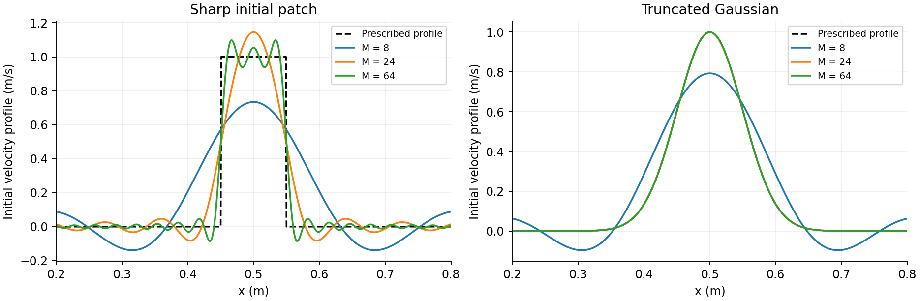One-dimensional factors in the initial-velocity expansion. The sharp cutoff produces Gibbs oscillations; the Gaussian is far easier to resolve. The full fields are products of these factors.

3. An independent finite-difference check

The finite-difference solver evaluates the displacement equations directly. It uses centred second differences for pure derivatives, the four-point centred stencil for mixed derivatives, and the central-time update

\[\mathbf u^{j+1}=2\mathbf u^j-\mathbf u^{j-1} +\Delta t^2\mathbf a_h(\mathbf u^j).\]

With $\mathbf u^0=0$, the initial acceleration vanishes and the startup is $\mathbf u^1=\Delta t\,\mathbf v_0$. The numerical solver uses no spectral derivatives and no modal frequencies.

It stores point values on a cell-centred grid, $x_i=(i+1/2)h$, rather than cell averages. At a wall, normal displacement is reflected oddly and tangential displacement evenly into ghost points. This enforces zero normal displacement and zero normal derivative of tangential displacement, consistent with the symmetry conditions. The Fourier reference is evaluated at the same physical points for error calculations.

For a $d$-dimensional grid, the runs use

\[\Delta t\leq\eta\frac{h}{\sqrt d\,c_P},\]

with $\eta=0.6$ in 2D and $0.7$ in 3D; the final step size is adjusted to hit the requested output time exactly. Both space and time are refined together, so the observed convergence is for the combined method.

A discontinuous patch is useful for reproducing the benchmark, but a smoother pulse makes convergence easier to interpret. For a Gaussian initial $x$ velocity with $\sigma=0.05$ m, centred at $(0.5,0.5)$ and truncated outside $[0.25,0.75]^2$, the results at $120\ \mu$s are:

Grid	Relative vector displacement error
$48^2$	5.54%
$96^2$	1.41%
$192^2$	0.353%

The finest refinement gives an observed order of approximately 2.00.

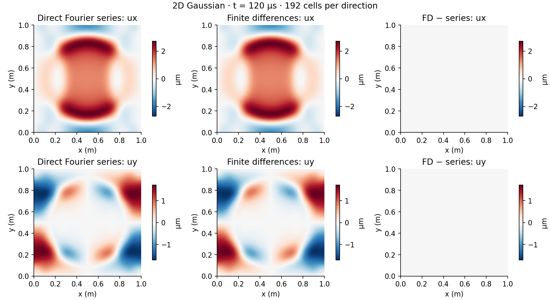The Fourier, FD and error panels use the same colour range within each component row.

4. The general framework

The steps we just followed can be stated without referring to potentials:

1. Choose a spatial basis compatible with the geometry and the boundary conditions.
2. Substitute the displacement expansion into the governing equations.
3. Use orthogonality to obtain equations for the time-dependent coefficients.
4. Diagonalise each independent modal block.
5. Determine its amplitudes from the initial conditions.
6. Reconstruct the field by summing the modes.

The special simplification in this box problem is not just that the basis satisfies the boundaries: the differential operator closes on a small component block for every spatial index. A boundary-compatible basis in a different problem may still yield a large coupled system.

For any nonzero wavevector, the elastic modal matrix has the structure

\[\mathbf H=\mu K^2\mathbf I+(\lambda+\mu)\mathbf k\mathbf k^T.\]

A vector parallel to $\mathbf k$ has eigenvalue $(\lambda+2\mu)K^2$. Every vector perpendicular to $\mathbf k$ has eigenvalue $\mu K^2$. This observation explains both the 2D result and its 3D extension.

5. Extend the same calculation to 3D

The three-dimensional calculation follows the same steps as the two-dimensional one. We add a coordinate $z$, a displacement component $u_z$ and a Fourier index $p$. The material law and sliding-wall conditions are the same.

Define the problem and expand displacement

Take a cube $\Omega=[0,L]^3$, with zero initial displacement and prescribed initial velocity $\mathbf v_0(x,y,z)$. On an $x$ face, impose $u_x=0$ and $\sigma_{xy}=\sigma_{xz}=0$; on a $y$ face, impose $u_y=0$ and $\sigma_{xy}=\sigma_{yz}=0$; on a $z$ face, impose $u_z=0$ and $\sigma_{xz}=\sigma_{yz}=0$.

Set

\[k_x=\frac{n\pi}{L},\qquad k_y=\frac{m\pi}{L},\qquad k_z=\frac{p\pi}{L}.\]

As in 2D, each displacement component uses a sine in its own direction and cosines in the other directions:

\[\begin{aligned} u_x&=\sum_{n=1}^{\infty}\sum_{m=0}^{\infty}\sum_{p=0}^{\infty} X_{nmp}(t)\sin(k_xx)\cos(k_yy)\cos(k_zz),\\ u_y&=\sum_{n=0}^{\infty}\sum_{m=1}^{\infty}\sum_{p=0}^{\infty} Y_{nmp}(t)\cos(k_xx)\sin(k_yy)\cos(k_zz),\\ u_z&=\sum_{n=0}^{\infty}\sum_{m=0}^{\infty}\sum_{p=1}^{\infty} Z_{nmp}(t)\cos(k_xx)\cos(k_yy)\sin(k_zz). \end{aligned}\]

The normal displacement vanishes on every face. The tangential shear tractions also vanish: for example, $\sigma_{xy}=\mu(u_{x,y}+u_{y,x})$ contains $\sin(k_xx)\sin(k_yy)$, while $\sigma_{xz}$ contains $\sin(k_xx)\sin(k_zz)$. Both are therefore zero on the $x$ faces. The other faces follow in the same way.

Substitute into the equations

The $x$ component of the governing equation now includes the $z$ derivatives:

\[\rho\ddot u_x =(\lambda+2\mu)u_{x,xx} +\mu(u_{x,yy}+u_{x,zz}) +(\lambda+\mu)(u_{y,xy}+u_{z,xz}).\]

For one triple $(n,m,p)$, temporarily suppress the mode indices. Differentiation gives

\[\begin{aligned} u_{x,xx}^{(nmp)}&=-k_x^2X\sin(k_xx)\cos(k_yy)\cos(k_zz),\\ u_{x,yy}^{(nmp)}&=-k_y^2X\sin(k_xx)\cos(k_yy)\cos(k_zz),\\ u_{x,zz}^{(nmp)}&=-k_z^2X\sin(k_xx)\cos(k_yy)\cos(k_zz),\\ u_{y,xy}^{(nmp)}&=-k_xk_yY\sin(k_xx)\cos(k_yy)\cos(k_zz),\\ u_{z,xz}^{(nmp)}&=-k_xk_zZ\sin(k_xx)\cos(k_yy)\cos(k_zz). \end{aligned}\]

Every term has the same spatial factor. Matching its coefficient, just as in 2D, gives the first equation below. Applying the same differentiation to the $y$ and $z$ components gives the other two:

\[\begin{aligned} \rho\ddot X +\big[(\lambda+2\mu)k_x^2+\mu(k_y^2+k_z^2)\big]X +(\lambda+\mu)k_xk_yY+(\lambda+\mu)k_xk_zZ&=0,\\ \rho\ddot Y +(\lambda+\mu)k_xk_yX +\big[(\lambda+2\mu)k_y^2+\mu(k_x^2+k_z^2)\big]Y +(\lambda+\mu)k_yk_zZ&=0,\\ \rho\ddot Z +(\lambda+\mu)k_xk_zX+(\lambda+\mu)k_yk_zY +\big[(\lambda+2\mu)k_z^2+\mu(k_x^2+k_y^2)\big]Z&=0. \end{aligned}\]

Recognise three coupled harmonic oscillators

The matrix form is

\[\rho \begin{bmatrix}\ddot X\\\ddot Y\\\ddot Z\end{bmatrix} +\mathbf H \begin{bmatrix}X\\Y\\Z\end{bmatrix} =\mathbf0,\]

where

\[\mathbf H= \begin{pmatrix} (\lambda+2\mu)k_x^2+\mu(k_y^2+k_z^2)&(\lambda+\mu)k_xk_y&(\lambda+\mu)k_xk_z\\ (\lambda+\mu)k_xk_y&(\lambda+2\mu)k_y^2+\mu(k_x^2+k_z^2)&(\lambda+\mu)k_yk_z\\ (\lambda+\mu)k_xk_z&(\lambda+\mu)k_yk_z&(\lambda+2\mu)k_z^2+\mu(k_x^2+k_y^2) \end{pmatrix}.\]

For positive $n,m,p$, this describes three coupled harmonic oscillators. The real symmetric positive-definite matrix has three independent normal modes. Before finding their frequencies, the general solution can be written as

\[\begin{aligned} X(t)&=\sum_{r=1}^{3}\big[A_{xr}\cos(\omega_rt)+B_{xr}\sin(\omega_rt)\big],\\ Y(t)&=\sum_{r=1}^{3}\big[A_{yr}\cos(\omega_rt)+B_{yr}\sin(\omega_rt)\big],\\ Z(t)&=\sum_{r=1}^{3}\big[A_{zr}\cos(\omega_rt)+B_{zr}\sin(\omega_rt)\big]. \end{aligned}\]

Here $r$ labels the three normal modes; it is separate from the spatial indices $(n,m,p)$. This component form has eighteen coefficient entries, whose relations will follow from the governing equations. There are six independent constants in total: one sine and one cosine amplitude per normal mode.

Find the frequencies and amplitude relations

Two time derivatives multiply each harmonic term by $-\omega_r^2$. Substituting into the matrix equation therefore gives, for each normal mode,

\[(\mathbf H-\rho\omega_r^2\mathbf I) \begin{bmatrix}A_{xr}\\A_{yr}\\A_{zr}\end{bmatrix}=\mathbf0, \qquad (\mathbf H-\rho\omega_r^2\mathbf I) \begin{bmatrix}B_{xr}\\B_{yr}\\B_{zr}\end{bmatrix}=\mathbf0.\]

This is the same amplitude equation as in 2D, with one additional row and column. Its determinant must vanish for a nonzero amplitude. With $K^2=k_x^2+k_y^2+k_z^2$, it factors as

\[\det(\mathbf H-\rho\omega^2\mathbf I) =\big[(\lambda+2\mu)K^2-\rho\omega^2\big] \big[\mu K^2-\rho\omega^2\big]^2=0.\]

The factorization follows from the matrix form given in the previous section, $\mathbf H=\mu K^2\mathbf I+(\lambda+\mu)\mathbf k\mathbf k^T$. It has one eigenvalue $(\lambda+2\mu)K^2$ and two equal eigenvalues $\mu K^2$.

Thus there are still only two distinct frequencies,

\[\omega_P=c_PK,\qquad \omega_S=c_SK,\]

with the same wave speeds as in 2D. The new feature is that two independent shear modes share $\omega_S$. Their sine terms can be combined, and their cosine terms can be combined. We can therefore write

\[\begin{aligned} X(t)&=A_{xP}\cos(\omega_Pt)+B_{xP}\sin(\omega_Pt) +A_{xS}\cos(\omega_St)+B_{xS}\sin(\omega_St),\\ Y(t)&=A_{yP}\cos(\omega_Pt)+B_{yP}\sin(\omega_Pt) +A_{yS}\cos(\omega_St)+B_{yS}\sin(\omega_St),\\ Z(t)&=A_{zP}\cos(\omega_Pt)+B_{zP}\sin(\omega_Pt) +A_{zS}\cos(\omega_St)+B_{zS}\sin(\omega_St). \end{aligned}\]

We now have twelve combined coefficients, four per displacement component. We determine their relations by substituting the two frequencies, exactly as in 2D.

For the $P$ cosine coefficients, the first row is

\[\begin{aligned} 0={}& \big[(\lambda+2\mu)k_x^2+\mu(k_y^2+k_z^2)-\rho\omega_P^2\big]A_{xP}\\ &+(\lambda+\mu)k_xk_yA_{yP} +(\lambda+\mu)k_xk_zA_{zP}. \end{aligned}\]

Since $\rho\omega_P^2=(\lambda+2\mu)K^2$, its diagonal bracket becomes $-(\lambda+\mu)(k_y^2+k_z^2)$. Dividing by $\lambda+\mu$ and collecting terms gives

\[\begin{aligned} -(k_y^2+k_z^2)A_{xP}+k_xk_yA_{yP}+k_xk_zA_{zP}&=0,\\ K^2A_{xP}&=k_x(k_xA_{xP}+k_yA_{yP}+k_zA_{zP}). \end{aligned}\]

The other two rows give the same relation with $x$ replaced by $y$ and $z$. For positive indices, comparing these three equations yields

\[k_yA_{xP}-k_xA_{yP}=0,\qquad k_zA_{xP}-k_xA_{zP}=0.\]

For the $S$ cosine coefficients, the first diagonal bracket instead becomes

\[(\lambda+2\mu)k_x^2+\mu(k_y^2+k_z^2)-\mu K^2 =(\lambda+\mu)k_x^2.\]

Its row therefore factors as

\[(\lambda+\mu)k_x (k_xA_{xS}+k_yA_{yS}+k_zA_{zS})=0.\]

The other rows have the same bracket, multiplied by $(\lambda+\mu)k_y$ or $(\lambda+\mu)k_z$. Hence

\[k_xA_{xS}+k_yA_{yS}+k_zA_{zS}=0.\]

The sine coefficients satisfy the same matrix equations, giving

\[\begin{aligned} k_yB_{xP}-k_xB_{yP}&=0,\\ k_zB_{xP}-k_xB_{zP}&=0,\\ k_xB_{xS}+k_yB_{yS}+k_zB_{zS}&=0. \end{aligned}\]

There are three relations among the cosine coefficients and three among the sine coefficients. The twelve combined coefficients therefore contain six independent constants, as expected for three coupled oscillators.

Apply the initial displacement

At $t=0$, all sine terms vanish and all cosine terms equal one. Zero initial displacement requires

\[A_{xP}+A_{xS}=0,\qquad A_{yP}+A_{yS}=0,\qquad A_{zP}+A_{zS}=0.\]

As in 2D, the independent normal-mode contributions cannot cancel to give a zero displacement vector unless their cosine amplitudes all vanish. Therefore,

\[A_{xP}=A_{yP}=A_{zP}=A_{xS}=A_{yS}=A_{zS}=0.\]

The reduced solution is

\[\begin{aligned} X(t)&=B_{xP}\sin(\omega_Pt)+B_{xS}\sin(\omega_St),\\ Y(t)&=B_{yP}\sin(\omega_Pt)+B_{yS}\sin(\omega_St),\\ Z(t)&=B_{zP}\sin(\omega_Pt)+B_{zS}\sin(\omega_St). \end{aligned}\]

Six sine coefficients remain, linked by the three relations above. We determine their values from the initial velocity.

Apply the initial velocity

Differentiate the reduced solution in time:

\[\begin{aligned} \dot X(t)&=\omega_PB_{xP}\cos(\omega_Pt)+\omega_SB_{xS}\cos(\omega_St),\\ \dot Y(t)&=\omega_PB_{yP}\cos(\omega_Pt)+\omega_SB_{yS}\cos(\omega_St),\\ \dot Z(t)&=\omega_PB_{zP}\cos(\omega_Pt)+\omega_SB_{zS}\cos(\omega_St). \end{aligned}\]

Evaluating at $t=0$ gives

\[\begin{aligned} \dot X(0)&=\omega_PB_{xP}+\omega_SB_{xS},\\ \dot Y(0)&=\omega_PB_{yP}+\omega_SB_{yS},\\ \dot Z(0)&=\omega_PB_{zP}+\omega_SB_{zS}. \end{aligned}\]

Expand the prescribed initial velocity in the same spatial series:

\[\begin{aligned} v_{0x}&=\sum_{n=1}^{\infty}\sum_{m=0}^{\infty}\sum_{p=0}^{\infty} V_x^{nmp}\sin(k_xx)\cos(k_yy)\cos(k_zz),\\ v_{0y}&=\sum_{n=0}^{\infty}\sum_{m=1}^{\infty}\sum_{p=0}^{\infty} V_y^{nmp}\cos(k_xx)\sin(k_yy)\cos(k_zz),\\ v_{0z}&=\sum_{n=0}^{\infty}\sum_{m=0}^{\infty}\sum_{p=1}^{\infty} V_z^{nmp}\cos(k_xx)\cos(k_yy)\sin(k_zz). \end{aligned}\]

For positive $n,m,p$, the coefficients are

\[\begin{aligned} V_x^{nmp}&=\frac{8}{L^3}\int_0^L\int_0^L\int_0^L v_{0x}\sin(k_xx)\cos(k_yy)\cos(k_zz)\,dx\,dy\,dz,\\ V_y^{nmp}&=\frac{8}{L^3}\int_0^L\int_0^L\int_0^L v_{0y}\cos(k_xx)\sin(k_yy)\cos(k_zz)\,dx\,dy\,dz,\\ V_z^{nmp}&=\frac{8}{L^3}\int_0^L\int_0^L\int_0^L v_{0z}\cos(k_xx)\cos(k_yy)\sin(k_zz)\,dx\,dy\,dz. \end{aligned}\]

Comparing this series with the time derivative of the displacement series gives, for every triple $(n,m,p)$,

\[\begin{aligned} \omega_P^{nmp}B_{xP}^{nmp}+\omega_S^{nmp}B_{xS}^{nmp}&=V_x^{nmp},\\ \omega_P^{nmp}B_{yP}^{nmp}+\omega_S^{nmp}B_{yS}^{nmp}&=V_y^{nmp},\\ \omega_P^{nmp}B_{zP}^{nmp}+\omega_S^{nmp}B_{zS}^{nmp}&=V_z^{nmp}. \end{aligned}\]

This is precisely the 2D matching step with a third component.

Solve for the remaining coefficients

Suppress the mode indices again. We have three initial-velocity equations and three amplitude relations, giving six equations for the six sine coefficients.

Multiply the initial-velocity equations by $k_x,k_y,k_z$, respectively, and add:

\[\begin{aligned} &\omega_P(k_xB_{xP}+k_yB_{yP}+k_zB_{zP})\\ &\qquad+\omega_S(k_xB_{xS}+k_yB_{yS}+k_zB_{zS}) =k_xV_x+k_yV_y+k_zV_z. \end{aligned}\]

The shear bracket is zero. The $P$ amplitude equations give, for each component $i=x,y,z$,

\[K^2B_{iP}=k_i(k_xB_{xP}+k_yB_{yP}+k_zB_{zP}).\]

Combining these expressions gives

\[\begin{aligned} B_{xP}&=\frac{k_x(k_xV_x+k_yV_y+k_zV_z)}{\omega_PK^2},\\ B_{yP}&=\frac{k_y(k_xV_x+k_yV_y+k_zV_z)}{\omega_PK^2},\\ B_{zP}&=\frac{k_z(k_xV_x+k_yV_y+k_zV_z)}{\omega_PK^2}. \end{aligned}\]

Each shear coefficient then follows from its initial-velocity equation:

\[\begin{aligned} B_{xS}&=\frac{V_x-\omega_PB_{xP}}{\omega_S} =\frac{V_x-k_x(k_xV_x+k_yV_y+k_zV_z)/K^2}{\omega_S},\\ B_{yS}&=\frac{V_y-\omega_PB_{yP}}{\omega_S} =\frac{V_y-k_y(k_xV_x+k_yV_y+k_zV_z)/K^2}{\omega_S},\\ B_{zS}&=\frac{V_z-\omega_PB_{zP}}{\omega_S} =\frac{V_z-k_z(k_xV_x+k_yV_y+k_zV_z)/K^2}{\omega_S}. \end{aligned}\]

Substituting into the reduced solution gives the three time functions:

\[\begin{aligned} X(t)&=\frac{k_x(k_xV_x+k_yV_y+k_zV_z)}{K^2}\frac{\sin(\omega_Pt)}{\omega_P}\\ &\quad+\left[V_x-\frac{k_x(k_xV_x+k_yV_y+k_zV_z)}{K^2}\right]\frac{\sin(\omega_St)}{\omega_S},\\[6pt] Y(t)&=\frac{k_y(k_xV_x+k_yV_y+k_zV_z)}{K^2}\frac{\sin(\omega_Pt)}{\omega_P}\\ &\quad+\left[V_y-\frac{k_y(k_xV_x+k_yV_y+k_zV_z)}{K^2}\right]\frac{\sin(\omega_St)}{\omega_S},\\[6pt] Z(t)&=\frac{k_z(k_xV_x+k_yV_y+k_zV_z)}{K^2}\frac{\sin(\omega_Pt)}{\omega_P}\\ &\quad+\left[V_z-\frac{k_z(k_xV_x+k_yV_y+k_zV_z)}{K^2}\right]\frac{\sin(\omega_St)}{\omega_S}. \end{aligned}\]

Setting $k_z=V_z=0$ gives $Z=0$ and recovers the 2D expressions for $X$ and $Y$. For example,

\[V_x-\frac{k_x(k_xV_x+k_yV_y)}{k_x^2+k_y^2} =\frac{k_y(k_yV_x-k_xV_y)}{k_x^2+k_y^2},\]

which is exactly the shear numerator in the 2D formula.

Handle zero indices and reconstruct displacement

As in 2D, an identically zero sine means that displacement component is absent. Set $V_x^{0mp}=0$, $V_y^{n0p}=0$ and $V_z^{nm0}=0$. For each constant cosine factor in a velocity integral, replace its normalization $2/L$ by $1/L$: the prefactor is $8/L^3$ with no zero cosine indices, $4/L^3$ with one and $2/L^3$ with two.

The final amplitude formulas use $K^2$ rather than individual wavenumbers, so they also apply to these reduced cases. With two nonzero indices there are two active displacement components; with only one, there is a single longitudinal oscillator. Skip $(0,0,0)$, whose spatial displacement patterns all vanish.

Finally, restore the indices on $X_{nmp}(t),Y_{nmp}(t),Z_{nmp}(t)$ and substitute them into the displacement series:

\[\begin{aligned} u_x(x,y,z,t)&=\sum_{n=1}^{\infty}\sum_{m=0}^{\infty}\sum_{p=0}^{\infty} X_{nmp}(t)\sin(k_xx)\cos(k_yy)\cos(k_zz),\\ u_y(x,y,z,t)&=\sum_{n=0}^{\infty}\sum_{m=1}^{\infty}\sum_{p=0}^{\infty} Y_{nmp}(t)\cos(k_xx)\sin(k_yy)\cos(k_zz),\\ u_z(x,y,z,t)&=\sum_{n=0}^{\infty}\sum_{m=0}^{\infty}\sum_{p=1}^{\infty} Z_{nmp}(t)\cos(k_xx)\cos(k_yy)\sin(k_zz). \end{aligned}\]

The construction is the same as in 2D: the initial velocity supplies the Fourier coefficients, the coupled-oscillator equations determine their time evolution, and the spatial series reconstructs displacement.

6. A 3D Gaussian pulse and a numerical check

Use the same unit cube and material, but prescribe

\[\mathbf v_0(\mathbf x)= \begin{cases} \displaystyle (1,0,0)^T\exp\!\left[-\frac{\|\mathbf x-\mathbf x_c\|^2}{2\sigma^2}\right] \ \mathrm{m/s},&\mathbf x\in[0.25,0.75]^3,\\ \mathbf0,&\text{elsewhere}, \end{cases}\]

where $\mathbf x_c=(0.5,0.5,0.5)$ m and $\sigma=0.05$ m. The initial $y$ and $z$ velocities are zero; their later displacements generally are not, because the elastic equations couple the components.

This pulse is exactly zero near every wall. It is truncated at five standard deviations, so its maximum jump at the support boundary is $e^{-12.5}\approx3.73\times10^{-6}$ of the peak. It is therefore not globally smooth, although the cutoff is very small.

The Gaussian separates in the coordinates. For one coordinate, calculate

\[S_n=\frac{2}{L}\int_{q_a}^{q_b}g(q)\sin(k_nq)\,dq,\qquad C_n=\frac{2-\delta_{n0}}{L}\int_{q_a}^{q_b}g(q)\cos(k_nq)\,dq.\]

Then $V_x=S_nC_mC_p$ in our unit-amplitude case, and $V_y=V_z=0$. More generally, multiply the corresponding products by the prescribed velocity components. Changing the pulse changes these integrals; it does not change the frequencies or amplitude relationships. The code evaluates the Gaussian integrals using converged Gauss–Legendre quadrature.

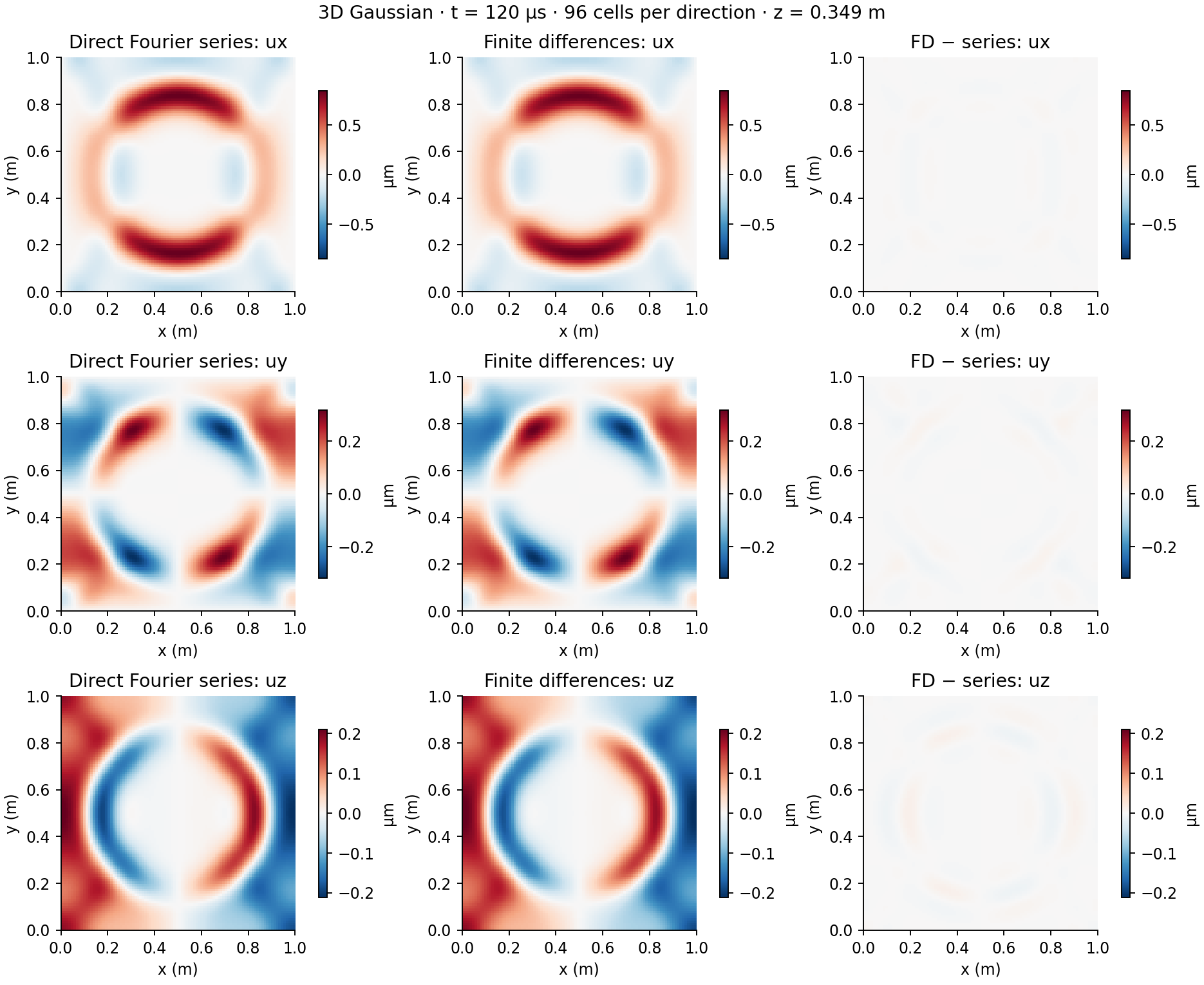At $120\ \mu$s, on the $96^3$ FD grid. An off-centre plane, $z\approx0.349$ m, exposes all three components. Each component row shares one colour scale across the reference, FD and difference panels.

Define the reported error by

\[\varepsilon_u= \left[\frac{\sum_{\text{grid points}}\|\mathbf u_{FD}-\mathbf u_{series}\|^2} {\sum_{\text{grid points}}\|\mathbf u_{series}\|^2}\right]^{1/2}.\]

This includes all three components and the full grid, not just the displayed slice.

Grid	Relative vector displacement error
$24^3$	28.39%
$48^3$	8.485%
$96^3$	2.194%

The last refinement has observed order 1.95, close to second order. The coarsest grid has only 1.2 cells per standard deviation and is poorly resolved. Increasing the series cutoff from 96 to 128 changes the reference by about $2.4\times10^{-8}$ in relative norm, well below the FD discrepancy. This is evidence of convergence, not a claim that the finest FD run is exact.

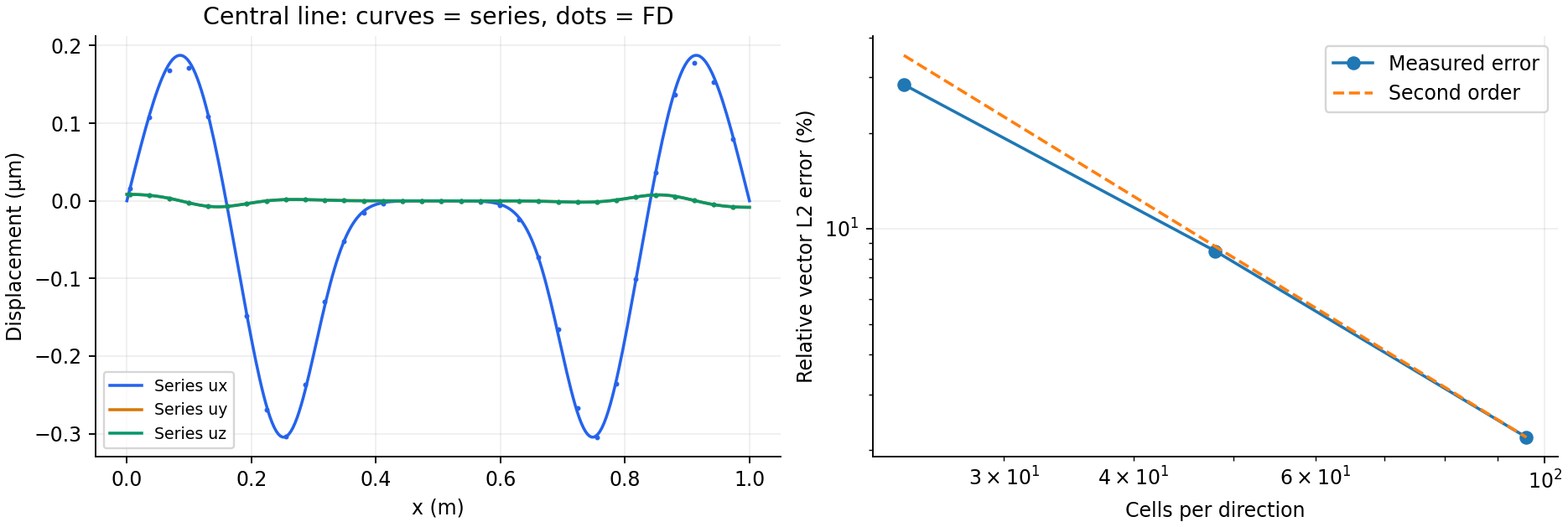Analytical line profiles include the physical boundaries. FD markers lie at cell centres. On an $x$ wall only $u_x$ must vanish; tangential components can move.

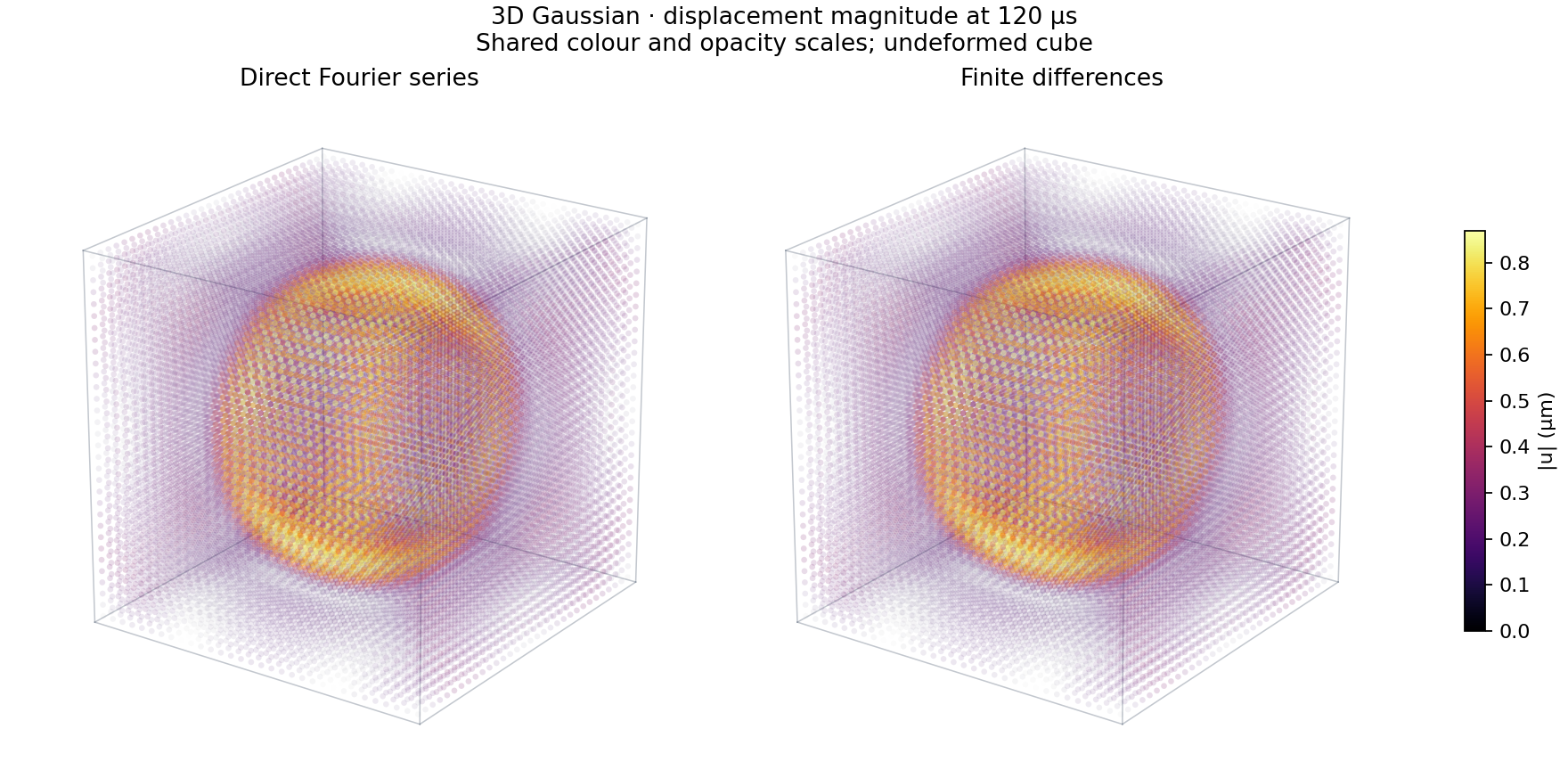
Sampled volume views of $|\mathbf u|$, with identical colour and opacity scales. Low displacement is transparent. The cube geometry is undeformed.

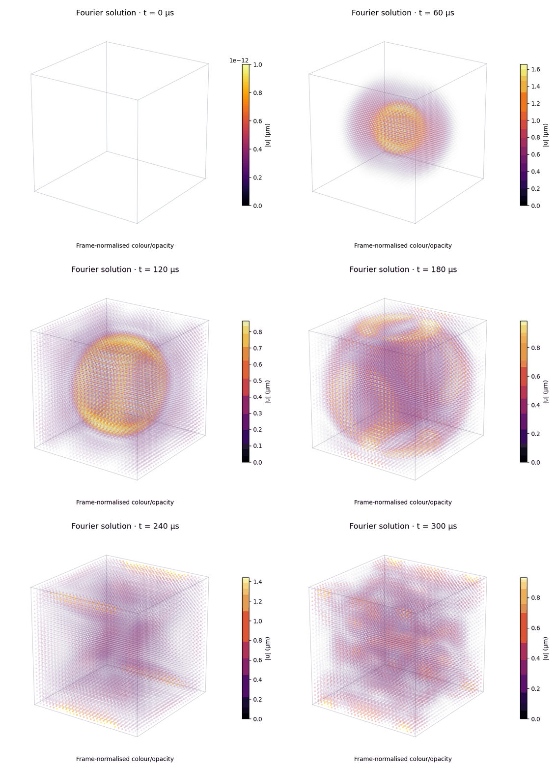Fourier-only displacement magnitude from $0$ to $300\ \mu$s. Colour and opacity are normalised separately in each frame so later fronts remain visible; the colour bar shows the current range. Brightness therefore cannot be compared across frames. The view uses 30 sampling points per axis and modes through index 48, not the grid used for the error table. A fixed-scale version is included in the source download.

Initially, the faster outer wavefront is longitudinal and the slower one is shear. For this material $c_P=2c_S$. From the pulse centre, their main arrivals at a face are approximately $79\ \mu$s and $158\ \mu$s, respectively. Reflected contributions then overlap. These are centre-to-wall travel times; the finite-width pulse has earlier, weaker arrivals.

7. What this gives WaveCore

For this box and these boundary conditions, the potential-free calculation is a short sequence: choose the spatial patterns, form the modal matrix, find its eigenstructure, and fit the initial velocity. The P/S split is still present physically; we have simply recovered it directly in displacement coordinates.

The derivation reproduces Chiappa’s 2D solution and extends through the same procedure to 3D. The accompanying FD checks give an independent numerical comparison. A Gaussian pulse is particularly useful when I want a clean convergence study rather than the high-frequency content of a sharp patch.

WaveCore already has a 2D Chiappa benchmark. Its 3D support is still developing. This solution provides a reference ready for that implementation, without pretending that the 3D FD results shown here were generated by WaveCore.

There was also an unexpected result: a displacement-magnitude isosurface from the 3D solution became the starting point for WaveCore’s logo. The geometry came from the wave field; the colours and lighting were chosen for the identity. A benchmark can be useful and rather beautiful at the same time.

Code and reproduction

View the complete examples repository on GitHub. It contains the direct solutions, a separate implementation of Chiappa’s Eqs. (23)–(27), the independent 2D/3D FD solver, tests, figure scripts and numerical results. It is standalone: WaveCore is not required to run these examples.

python -m venv .venv
# Linux/macOS; on Windows activate .venv\Scripts\Activate.ps1 instead
source .venv/bin/activate
python -m pip install -e '.[test]'
OPENBLAS_NUM_THREADS=1 python -m pytest -q
OPENBLAS_NUM_THREADS=1 python examples/reproduce.py --case all
OPENBLAS_NUM_THREADS=1 python examples/visualize.py --animate --adaptive

The scripts operate in SI units and include constant-cosine modes correctly. All comparison figures are newly generated; the publication’s copyrighted PDF and original figures are not redistributed. Machine-readable parameters, cutoffs and errors accompany the figures.

Reference

[1] A. Chiappa, S. Iakovlev, A. Marzani, F. Giorgetti, C. Groth, S. Porziani and M. E. Biancolini, An analytical benchmark for a 2D problem of elastic wave propagation in a solid, Engineering Structures 229 (2021), 111655. doi:10.1016/j.engstruct.2020.111655.