From small principles to big structures: modelling hanging cables.
Introduction
I remember my first walk in one of the residential neighbourhoods of Oxford. One of the things that most struck me were the electric hanging cables from wooden poles.
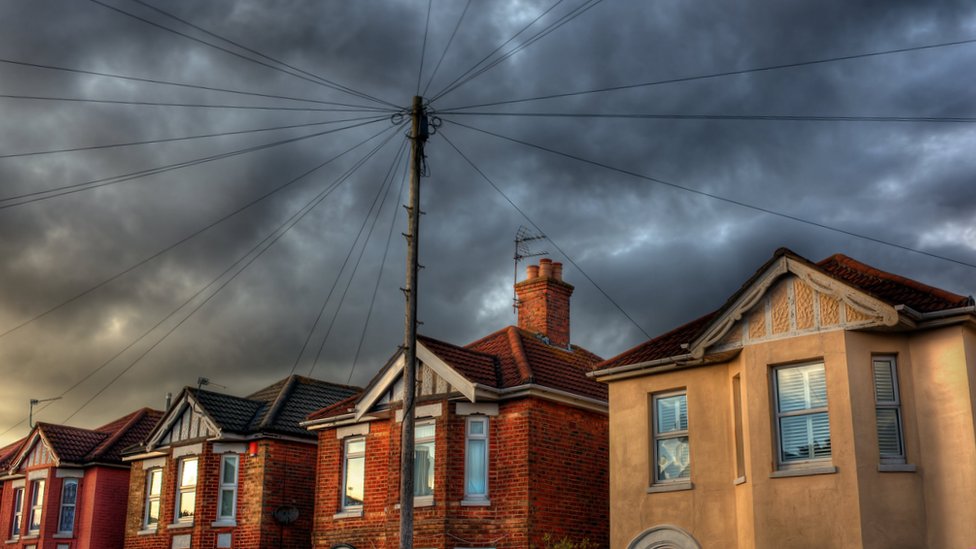
This intricate web of hanging wires over my head caught my imagination at the time, and still does today.
The scientific debate on the shape that cables take as a result of gravity has span centuries, with contribution from Galileo to Bernoulli.
For a long time it was taught that hanging cables would form parabolas, but a rigorous analysis of the problem from Bernoulli showed that indeed the shape is a hyperbolic cosine, since then called catenary. proof
The analysis is formally correct however is limited to cables with constant mass, and is not simply applicable to webs, and more complicated problems like varying mass etc.
Thankfully we now live the mighty era of computers, and in this post I will outline a strategy able to model hanging cables, using first principles.
I will first break down the problem in small atomic units, that when put together will result in catenaries.
The physical model
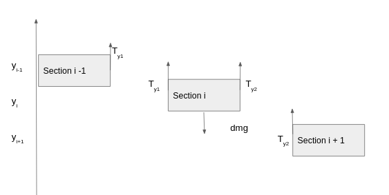
In absence of wind and other forces a cable hanging between 2 points A and B is at rest. This is a result of the first principle of dynamics by Newton. In simpler terms, the resultant of the forces acting on any section of the cable however small is zero:
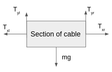
In equation format:
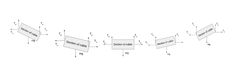
\[\sum F_x = T_{xr} - T_{xl} = 0\] \[\sum F_y = T_{yr} + T_{yl} - mg = 0\]These two equation basically say the the tensions in the cable have to equilibrate the mass of that section. Now that we have a simple understanding, of how a section of behaves, we can slice up the whole cable and for every section draw the tensions and the weights.
The weight force
If we have a cable of initial length \(L\) we can divide it in \(n\) elements of length \(dl = \frac{L}{n}\) if we imagine the linear density of the cable to be constant \(\rho\) Every element will have a mass of
\[dm = \rho * dl\]Therefore the weight acting on every section of the cable will be
\[dw = dm * g\]The tension force
If you take a cable and try to stretch it, you will feel a resisting force in your arm, that is the cable tension. We will make the simplest assumption, that is that if double the force, you will feel twice the resistance from the cable, i.e. the cable has a linear response.
\[T_x = k * l_x\] \[T_y = k * l_y\]The equations above tell us that if we apply a force on a cable of inital length $l$ it will resist with a force equal and opposite. This force is proportional to the material property $k$, the higher this constant the smaller the material stretch. In the equations above $l_x$ and $l_y$ are the lengths in the $x$ and $y$ direction. In this simulation they will be the $x$ and $y$ coordinates of two consecutive sections of the cable.
This type of spring is called a zero length spring.
Connecting two springs
At any internal section of the cable we will have two forces coming from the left and the right spring, so for a movement in the positive $x$ direction of a cable section the equilibrium will be:
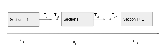
At the same time in the y direction:
Solving the problem
Armed with $\eqref{1}$ and $\eqref{2}$ we can now solve the problem of finding the shape of a cable under its own weight.
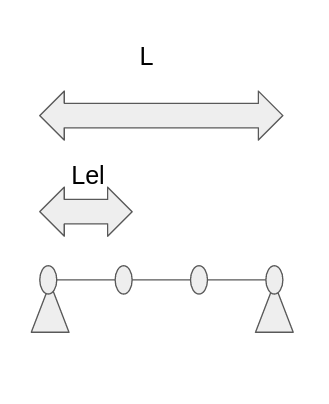
We define a cable of lenght $L$, discretized with $N$ elements of length $L_{el}$ in a straigth position, at $y=0$. The cable has a stiffnes $k$ and a density $\rho$. Obviously in this starting position the equilibrium is not respected and equation $\eqref{2}$ will have a non-zero value.
Our intuitiution is that we need to pull the cable down to generate a force equal and opposite to the weight of the cable, however how do we define this amount of displacement?
One way to do it, would be to randomly assign a position to every section of the cable, and hope for the best, however there is a clever way to go about it.
Optimization using gradient descent
As a recap, our objective is to find for every section of the cable a position $(x,y)$ such that the elastic force of the cable is in static equilibrium with the weight of the cable.
So given a configuration we can define the error as:
\[\sum^{n - 1 }_{1}(k * x_{i - 1} -2 * k * x_i - k * x_{i + 1})^2 + (k * y_{i - 1} -2 * k * y_i + k * y_{i + 1} - dm*g)^2 = E \tag{3}\label{3}\]In $\eqref{3}$ $E$ is the level of error. The error is 0 if and only if the two contributions are 0, which means that equation $\eqref{1}$ and $\eqref{2}$ are satisfied. The sum runs over the internal nodes of the cable since the boundaries are fixed.
To minimize the error we will use a gradient descent approach, i.e.
- Compute $\frac{\partial{E}}{\partial{x_i}}$ and $\frac{\partial{E}}{\partial{y_i}}$
- Update $x_i = x_i - \eta * \frac{\partial{E}}{\partial{x_i}}$
- Update $x_i = y_i - \eta * \frac{\partial{E}}{\partial{y_i}}$
- Repeat
In the algorithm above $\eta$ is a user defined parameter and
\[\frac{\partial{E}}{\partial{x_i}} = -4 * k * (k * x_{i - 1} -2 * k * x_i - k * x_{i + 1})\] \[\frac{\partial{E}}{\partial{y_i}} = -4 * k * (k * y_{i - 1} -2 * k * y_i + k * y_{i + 1} - dm*g)\]The code
For this project I have used C++ to solve the catenary problem, the code is hosted on my github . At the hearth of the algorithm we will use, there are 3 functions I will post here for convenience.
1
2
3
4
5
6
7
8
9
10
11
12
13
14
void updateForces(const std::vector<Vec2D>& positions,
                  const std::vector<scalar>& mass,
                  const scalar K,
                  const scalar gravity,
                  std::vector<Vec2D>& forces){

    for (int i = 1; i < forces.size() - 1; ++i){
        forces[i].x = (positions[i - 1].x - 2 *positions[i].x  + positions[i + 1].x ) * K;

        forces[i].y = (positions[i - 1].y - 2*positions[i].y  + positions[i + 1].y ) * K - mass[i] * gravity;

    }

}
In updateForces we will update the forces vector given the position, mass, stiffness and gravity.
1
2
3
4
5
6
7
8
9
10
scalar getResidual(const std::vector<Vec2D>& forces){

    scalar res = 0;

    for (size_t i = 1; i < forces.size() - 1; ++i){
        res += norm(forces[i]);
    }

    return res;
}
Once the forces have been computed we have to understand wheter we are in static equilibrium $\eqref{3}$. I used a typedef scalar to experiment with different precisions.
Finally we can compute the derivates of the error with respect to the positions $x$ and $y$ of every node using
1
2
3
4
5
6
7
8
9
10
11
12
13
std::vector<Vec2D> getDerivatives(const std::vector<Vec2D>& positions,
                  const std::vector<scalar>& mass,
                  const scalar K,
                  const scalar gravity) {

std::vector<Vec2D> derivatives;

 for (int i = 1; i < positions.size() - 1; ++i){
    derivatives.emplace_back(Vec2D{-4 * (positions[i - 1].x - 2 *positions[i].x  + positions[i + 1].x ) * K,
                                   -4 * ( (positions[i - 1].y - 2 *positions[i].y  + positions[i + 1].y ) * K - mass[i] * gravity)});
 }
    return derivatives;
}
So the algorithm will work as follows:
- Define inputs
- Start from straight cable
- Call
updateForces - Call
getResidual - If residual is bigger then threshold, continue else end.
- Call
getDerivatives - Update Positions
- Repeat
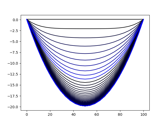
For fun, here is the static image of the algorithm converiging to the final position of the cable, using data from this video
Conclusions
We have delved into the physical world around us, and examined how a structure like a cable under its own weight, can be modelled using first principles and atomic elements. Thank to the power of computers, this kind of approach in very popular in simulations, since it is simple and explainable.
We then have solved numerically the static equilibrium of the cable using gradient descent, a popular algorithm used in ML domain. Finally we have coded up the algorithm from scratch and compared the result against the analytical solution with a good degree of approximation.
I hope you had as much fun reading this as I had coding and writing this up.